
Targeting and supertargeting#
The chapters before this one judged a network by one pair of numbers, the
minimum energy requirement (MER) targets of its problem table. Pinch analysis
can say much more before a single exchanger exists: how the heating and
cooling targets split between several utilities and what they cost, how much
exchanger area and how many units a network of these streams needs, what
that area costs, and therefore which T_min_app minimizes the total
annualized cost. hensmith.targeting computes all of these
(PinchTargets), sweeps T_min_app for the least total
annualized cost (supertarget()), draws the composite curves,
the grand composite curve and the sweep, and compares a synthesized network
with its targets (network_report()).
Every number and figure below is output of the code shown on this page. The quickstart system built here is chapter 1’s build repeated verbatim, so this page runs on its own.
Imports and the system#
import numpy as np
import matplotlib.pyplot as plt
from hensmith import (supertarget, network_report, plot_composite_curves,
                      plot_grand_composite_curve, plot_supertargets)
import biosteam as bst
from hensmith import HeatExchangerNetwork

bst.settings.set_thermo(['Water', 'Methanol', 'Glycerol'], cache=True)
bst.main_flowsheet.set_flowsheet('quickstart')
feed1 = bst.Stream('feed1', flow=(8000, 100, 25))
feed2 = bst.Stream('feed2', flow=(10000, 1000, 10))
D1 = bst.ShortcutColumn('D1', ins=feed1,
                        outs=('distillate', 'bottoms_product'),
                        LHK=('Methanol', 'Water'),
                        y_top=0.99, x_bot=0.01, k=2,
                        is_divided=True)
D1_H1 = bst.HXutility('D1_H1', ins=D1.outs[1], T=300)
D1_H2 = bst.HXutility('D1_H2', ins=D1.outs[0], T=300)
F1 = bst.Flash('F1', ins=feed2, outs=('vapor', 'liquid'), V=0.9, P=101325)
HXN = HeatExchangerNetwork('HXN', T_min_app=5.)
sys = bst.System.from_units('sys', units=[D1, D1_H1, D1_H2, F1, HXN])
sys.simulate()
The facility’s targets#
HXN.targets() returns the
targets of the streams the facility synthesized from, in its stream order and
at its T_min_app (or at another one, HXN.targets(10.), without
synthesizing anything).
targets = HXN.targets()        # the facility's streams at its T_min_app
print(targets)
print('streams:', targets.labels)
print(f'shifted pinch: {targets.pinch_T:.2f} K')
info = HXN.synthesis_info
print('equal to the synthesis targets:',
      targets.Q_hot == info['Q_hot_target'], targets.Q_cold == info['Q_cold_target'])
print(f'heating utility of the network: {HXN.actual_heat_util_load:.4g} kJ/hr')
<PinchTargets: 5 streams, T_min_app = 5 K, Q_hot = 2.828e+08 kJ/hr, Q_cold = 1.936e+06 kJ/hr>
streams: ['D1 - reboiler', 'F1 - heat_exchanger', 'D1_H1', 'D1 - condenser', 'D1_H2']
shifted pinch: 298.15 K
equal to the synthesis targets: True True
heating utility of the network: 2.977e+08 kJ/hr
The streams are labeled by their units, an auxiliary exchanger by its owner and its own ID. The targets are the synthesis’s own, bit for bit: the facility prepares the streams for targeting exactly as the synthesis prepares them. They are process side: 2.828e+08 kJ/hr is the heat the cold streams need from a hot utility. The network’s heating load, 2.977e+08 kJ/hr here and in Configuring the network and a larger system, is utility side: biosteam divides each duty by its agent’s heat transfer efficiency, 0.95 for steam, and 2.828e+08 / 0.95 is 2.977e+08.
Nothing is stored on the facility, and nothing is re-synthesized: the targets
are those of the units’ current states, which, with cache_network=True,
can differ from the cached network’s. Each stream runs from its unit’s inlet
now to its outlet as the unit was last simulated, so after a feed changes,
simulate the system (or the units) before targeting: a stream whose inlet has
changed in flow since warns that its targets mix the new inlet with the former
outlet, a state of no process. The streams themselves are those of the
facility’s last simulation, one per heat utility its units listed then: a unit
in parallel simulated alone that changes its number of units (a fermentor’s
parallel['self'], set by its volume) warns, as biosteam lists its heat
utilities once per unit, until the system is simulated. The same object can be
built without a facility, from the heat utilities of heat exchangers with
PinchTargets.from_heat_utilities
(as the trade-off example below does) or from streams as
problem_table() takes them. The facility’s selection,
bst.process_tools.heat_exchanger_utilities_from_units(sys.units), is the
one to give it: a heat utility that a unit adds for itself (a reactor’s or a
heated mixer’s, hu.hxn_ok False) raises a ValueError, as its unit’s
first inlet and outlet need not be the stream it heats or cools. A selection
is valid until its units are simulated again: biosteam then gives each unit
new heat utilities, emptying the former ones, so select them again after any
simulation (a former one, no longer among its unit’s heat_utilities,
raises a ValueError rather than drop out as a heat utility without duty).
A heat utility counts as a stream each time it is given, as in the synthesis:
biosteam lists the heat utility of a unit in parallel once per unit (a
fermentor’s recirculation cooler, for one, once per reactor of its
parallel['self']), and so does the selection. One given more often than
its unit and owners list it, as selections from overlapping unit lists (a
unit and an auxiliary unit of it) give it, raises a ValueError: its
stream would count once more per extra one. Given
key_units=sys.units too, the keys of approach_contributions and of
h may name any unit, as the facility’s may: 'K1' then covers the
intercoolers of a biosteam.MultistageCompressor K1, which builds them
without an owner. After a simulation with replace_unit_heat_utilities=True,
though, the units’ heat utilities hold the network’s utilities, not the
process duties, and those of the streams that the process exchangers serve
completely are empty: the selection then gives the wrong streams (with a
RuntimeWarning), and HXN.targets() is the one to take.
Several utilities on the grand composite curve#
The MER targets say how much heating and cooling the streams need, not which
utilities supply them. utility_targets() places
biosteam’s heating and cooling agents on the grand composite curve,
following biosteam’s own rules for which agent may serve which temperature,
and prices each with biosteam.
utilities = targets.utility_targets()     # biosteam's default agents
print('agent               duty        utility duty  level   process T [K]     cost')
print('                    [kJ/hr]     [kJ/hr]       [K]     in -> out         [USD/hr]')
for u in utilities:
    print(f'{u.ID:<18}  {u.duty:<10.4g}  {u.utility_duty:<12.4g}  {u.level:<6.2f}  '
          f'{u.T_in:.2f} -> {u.T_out:.2f}  {u.cost:.2f}')
print(f'utility cost target: {sum(u.cost for u in utilities):.2f} USD/hr')
for u in utilities:
    print(f'{u.ID}: {u.flow:.4g} kmol/hr, from {u.T_utility_in:.2f} to {u.T_utility_out:.2f} K')
agent               duty        utility duty  level   process T [K]     cost
                    [kJ/hr]     [kJ/hr]       [K]     in -> out         [USD/hr]
low_pressure_steam  2.828e+08   2.977e+08     407.19  298.15 -> 372.60  1829.93
chilled_water       1.936e+06   1.936e+06     282.37  303.15 -> 300.00  9.68
utility cost target: 1839.61 USD/hr
low_pressure_steam: 7695 kmol/hr, from 412.19 to 412.19 K
chilled_water: 1443 kmol/hr, from 280.37 to 298.15 K
Each agent has a level on the shifted scale: the warmest temperature it
can serve, or the coldest, for a coolant. A heating agent’s level is its
temperature less biosteam’s approach, the agent’s own dT plus
HeatUtility.dT: 412.19 - 0 - 5 = 407.19 K for low pressure steam. A
coolant’s level is its temperature plus that approach, moved onto the shifted
scale by subtracting T_min_app, the hot streams’ shift:
280.37 + 2 + 5 - 5 = 282.37 K for chilled water. Low pressure steam, first in
biosteam’s list of heating agents, is above the top of the cold streams, so it
takes the whole hot utility target; a hotter steam would only be used for what
it cannot serve.
Every cold stream above the pinch is heated by it, from 298.15 K (the pinch)
to 372.60 K, and biosteam prices that duty at 1829.93 USD/hr, with the same
division by the heat transfer efficiency as in the network: the utility duty
is 2.977e+08 kJ/hr. On the cold side, cooling water, the first coolant in the
list, gets nothing: all the cold utility is needed below 303.15 K (30 °C, the
pinch on the hot streams’ scale), colder than cooling water can serve. Chilled
water serves it. A sensible agent, it enters at 280.37 K and leaves at 298.15
K, 5 K below the warmest process temperature it serves, 303.15 K: biosteam
limits a sensible agent’s outlet at that end, and hensmith also keeps its
line 5 K from the process across the whole stretch, which here allows the
same outlet (a condenser at the cold end of the stretch would hold it lower).
The utility cost target, 1839.61 USD/hr, is the cost of the MER utilities
with biosteam’s agents placed this way.
The grand composite curve shows the allocation: each agent is a horizontal segment at its level, as wide as its duty, the heating ones from the lowest level up, each starting where the one below ends, and the cooling ones mirrored below the pinch.
fig, ax = plot_grand_composite_curve(targets, utilities=utilities)
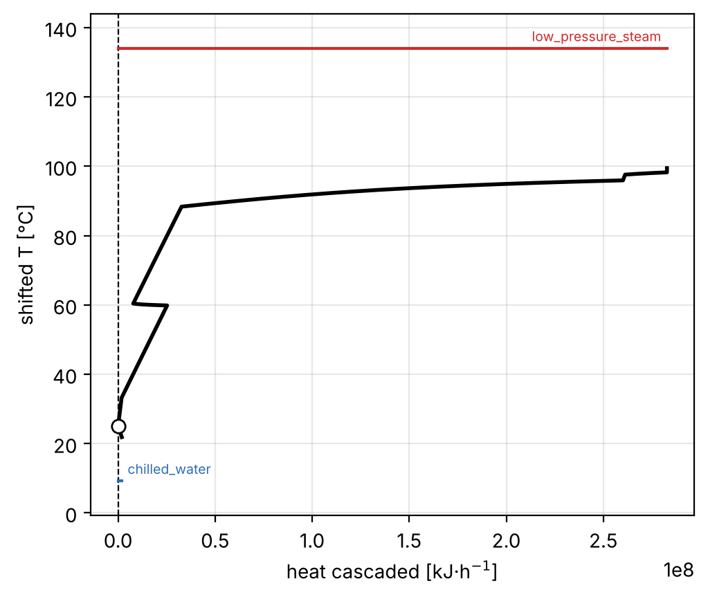
The grand composite curve of the quickstart system at T_min_app = 5 K
(the same curve as chapter 2’s), with the utility targets as a staircase:
low pressure steam at its level, 407.19 K (134 °C on the shifted scale),
serves all 2.828e+08 kJ/hr of the hot utility target, above every cold
stream; chilled water at 282.37 K serves the 1.936e+06 kJ/hr of cold
utility below the pinch. The open circle is the pinch, 298.15 K shifted.#
Composite curves, plain and balanced#
Chapter 2 drew the composite curves from the fields of a
ProblemTable in its own script;
plot_composite_curves() draws them from the targets, and
composite_curves() returns their points. With
kind='balanced' the utilities join the curves: the heating utilities the
hot composite and the cooling ones the cold composite, so that both curves end
at the same heat. These balanced composite curves are what the area
target below is computed on.
fig, ax = plot_composite_curves(targets)
fig_balanced, ax_balanced = plot_composite_curves(targets, kind='balanced',
                                                  utilities=utilities)
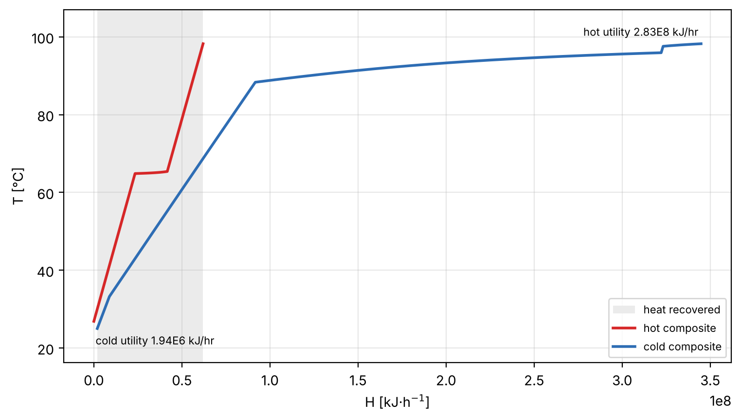
The composite curves of chapter 2, drawn by the library: the shaded band is the heat recovered, the cold composite starts at the cold utility target, 1.936e+06 kJ/hr, and ends the hot utility target, 2.828e+08 kJ/hr, beyond the end of the hot one. The script checks that their knots are chapter 2’s.#
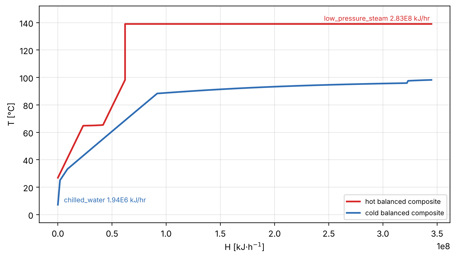
The balanced composite curves. The steam condenses at 412.19 K, so it is a flat at that temperature (139 °C), 2.828e+08 kJ/hr long, at the warm end of the hot curve; chilled water warms from 280.37 to 298.15 K, a line at the cold end of the cold curve, 1.936e+06 kJ/hr long. Both curves now span the same heat; the area target assumes that every bit of it is transferred vertically, from the hot curve to the cold curve below it.#
Area, units, capital and total cost#
On the balanced composite curves, summary()
targets the rest of the cost of a network. The methods that take
utilities need those of the same targets: a list from targets at another
T_min_app (targets.at(20.), say) or a part of one would not balance
the curves, so its duties are checked against Q_hot and Q_cold, and
the shifted temperatures its levels are on (each utility’s shift) against
the targets’ shift; a mismatch raises a ValueError.
print('units:', targets.units_target(utilities))
capital = targets.capital_cost_target(utilities)
print(f"{capital['N_area_shells']} of {capital['N_shells']} shells share the area: "
      f"{capital['shell_area']:.4g} m2 each, {capital['type']}")
summary = targets.summary()     # 10 % over 10 years; 8000 h/yr (no system hours)
for key, value in summary.items():  # numbers, and the shell type
    print(f'{key:<24} {value}' if isinstance(value, str) else f'{key:<24} {value:.6g}')
units: {'above': 5, 'below': 1, 'total': 6}
6 of 6 shells share the area: 991 m2 each, Floating head
T_min_app                5
Q_hot                    2.82781e+08
Q_cold                   1.93588e+06
utility_cost             1839.61
area                     5946.13
N_units                  6
N_shells                 6
N_area_shells            6
shell_area               991.022
shell_type               Floating head
purchase_cost            710660
installed_cost           2.28172e+06
annualized_capital_cost  371339
operating_cost           1.47169e+07
TAC                      1.50882e+07
Area, 5946.13 m²: Bath’s formula, the area of an ideal network that transfers heat vertically between the balanced composite curves, each stretch between their breakpoints at its log-mean temperature difference and each stream’s share of it over its own film coefficient. By default every stream and utility has a film coefficient of 1 kW/m²/K, so any pair has biosteam’s heuristic overall coefficient of 0.5 kW/m²/K;
h=andh_utilities=give streams and agents their own.Units, 6 (5 above the pinch and 1 below): Euler’s rule, the number of streams and utilities less one, in each region between the zeros of the balanced grand composite curve. It is an estimate, not a bound: a subset of streams that balances on its own needs fewer units.
Capital: the area divided into as many shells of equal area as there are units, here 6 floating head shells of 991 m², each costed with biosteam’s own correlations: 2.28172e+06 USD installed. When the equal shells would fall below 150 ft² (14 m²), where biosteam’s double pipe costs a fraction of a shell and tube, the target keeps the shell and tubes the area fills if they cost more (see Key Concepts);
'N_area_shells','shell_area'and'shell_type'say which shells carry the area.Total annualized cost (TAC), 1.50882e+07 USD/yr: the installed cost times the capital recovery factor (371339 USD/yr: 10 % interest over 10 years by default) plus the utility cost times the operating hours (1.47169e+07 USD/yr: 8000 h/yr by default). It counts the bare module cost of the exchangers only, no Lang factor and no working capital.
interest=,years=andoperating_hours=change the economics, ortea=takes them from a biosteam TEA. The facility’s targets know their system: if it has operating hours (a TEA sets them), the summary and the sweep below use them instead of 8000 h/yr. The quickstart system has none.
Supertargeting: the least total annualized cost#
Chapter 4 swept T_min_app by synthesizing a network at each value.
supertarget() sweeps the targets instead: it reuses the
streams’ curves, so no stream is flashed again, and evaluates the summary at
each T_min_app, then refines the grid around the least TAC. Each point
still builds its own problem table, which reads every stream’s enthalpy on the
grid; on a system of many streams with rigorous thermodynamics, a sweep of the
default 40 points and three refinements can take longer than a synthesis, and
a coarser T_min_apps or a smaller refine keeps it short.
sweep = supertarget(targets, np.arange(1., 31.))
print(sweep)
print('T_min_app  Q_hot      Q_cold     area    units  installed  capital    operating  TAC')
print('[K]        [kJ/hr]    [kJ/hr]    [m2]           [USD]      [USD/yr]   [USD/yr]   [USD/yr]')
optimum = sweep.optimum
after = sweep.records[sweep.records.index(optimum) + 1]     # the next point evaluated
for r in sweep.records:
    if r['T_min_app'] in (1., 2., 5., 10., 15., 20., 25., 30.) or r is optimum or r is after:
        print(f"{r['T_min_app']:<9.4g}  {r['Q_hot']:<9.4g}  {r['Q_cold']:<9.4g}  "
              f"{r['area']:<6.0f}  {r['N_units']:<5d}  {r['installed_cost']:<9.4g}  "
              f"{r['annualized_capital_cost']:<9.4g}  {r['operating_cost']:<9.4g}  {r['TAC']:.0f}")
print(f'optimum {sweep.T_min_app:.4g} K, at the bound of the sweep: {sweep.at_bound}')
fig, ax = plot_supertargets(sweep)
<Supertargets: 54 points, T_min_app 1-30 K, optimum 1.849 K (TAC 1.494e+07 USD/yr)>
T_min_app  Q_hot      Q_cold     area    units  installed  capital    operating  TAC
[K]        [kJ/hr]    [kJ/hr]    [m2]           [USD]      [USD/yr]   [USD/yr]   [USD/yr]
1          2.808e+08  0          6836    5      2.482e+06  4.04e+05   1.454e+07  14943217
1.849      2.808e+08  0          6836    5      2.482e+06  4.04e+05   1.454e+07  14943211
1.853      2.808e+08  2049       6835    6      2.555e+06  4.158e+05  1.454e+07  14955188
2          2.809e+08  9.219e+04  6759    6      2.532e+06  4.12e+05   1.455e+07  14959665
5          2.828e+08  1.936e+06  5946    6      2.282e+06  3.713e+05  1.472e+07  15088200
10         2.859e+08  5.009e+06  5440    6      2.127e+06  3.461e+05  1.5e+07    15344973
15         2.9e+08    9.138e+06  5158    9      2.269e+06  3.693e+05  1.533e+07  15694680
20         2.975e+08  1.662e+07  5073    9      2.243e+06  3.651e+05  1.573e+07  16093036
25         3.049e+08  2.41e+07   5042    9      2.234e+06  3.635e+05  1.613e+07  16498447
30         3.124e+08  3.157e+07  5042    9      2.234e+06  3.635e+05  1.654e+07  16904956
optimum 1.849 K, at the bound of the sweep: False
The quickstart system is dominated by steam: its operating cost, 1.454e+07 to
1.654e+07 USD/yr over the sweep, is about forty times its annualized capital
cost, so the TAC follows the utility cost and falls as T_min_app does. Below
about 1.85 K the system is a threshold problem: it needs no cold utility at
all, so the hot utility, its steam and the balanced composite curves no longer
change with T_min_app, and neither does any target. The TACs at 1 and at
1.849 K differ by less than 7 USD/yr, 4e-7 of the TAC, which is no physical
effect: the problem table’s grid moves with T_min_app over the curved
(vapor-liquid) profiles of the streams, and the area follows it, too little
to show in the table (6836 m² at both). Every T_min_app of that flat
stretch is an optimum but for these few USD/yr. The area, and with it the TAC,
falls steadily across the stretch as the grid moves, so the least TAC is always
the warmest point evaluated below the threshold, here 1.849 K (inside the
sweep, not at its bound), 0.004 K short of the step. That step comes at the
next point, 1.853 K: the cold utility appears and needs a unit of its own (6
units), which adds about 12000 USD/yr to the TAC. Between 10 and 15 K, where
chapter 4’s sweep saw the pinch move to the column condenser’s vapor inlet,
the units target jumps to 9.
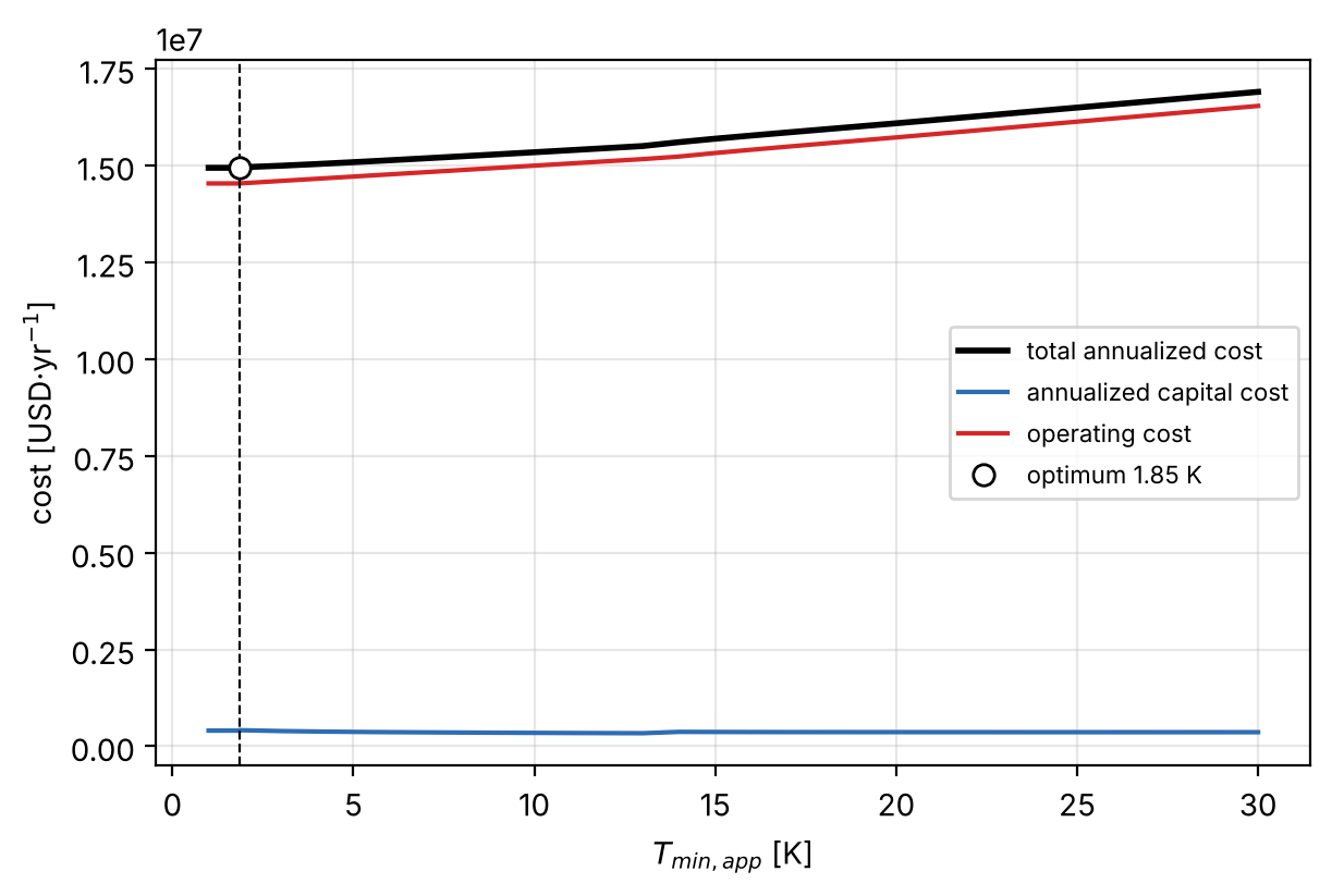
The sweep of the quickstart system. The total annualized cost (black) is the operating cost (red) plus the annualized capital cost (blue); the circle and the dashed line mark the least TAC, 1.494e+07 USD/yr at 1.849 K. Capital is a small fraction of the TAC, so the optimum has the least utility: it is on the flat stretch below 1.85 K, where no cold utility (and no unit for it) is needed, and any point of that stretch would do.#
A trade-off between capital and energy needs a system whose capital
matters. The two streams below, a hot and a cold one of 100 kW/K each, are
served by steam at 450 K and by water evaporating at 280 K, two latent agents
made for the example with prices of 4e-7 and 2e-7 USD/kJ. Their targets come
straight from their heat utilities with
PinchTargets.from_heat_utilities,
and heating_agents= and cooling_agents= are passed on to every summary
of the sweep.
import thermosteam as tmo
from hensmith import PinchTargets
fluid = tmo.Chemical('Fluid', search_db=False, phase='l', MW=1.,
                     Cn=3.6, default=True)     # 1000 kmol/hr: 1 kW/K
bst.settings.set_thermo([fluid])
bst.main_flowsheet.set_flowsheet('trade_off')
H1 = bst.HXutility('H1', ins=bst.Stream('H1_in', Fluid=1e5, T=400.),
                   T=320., rigorous=False)       # 100 kW/K, 400 -> 320 K
C1 = bst.HXutility('C1', ins=bst.Stream('C1_in', Fluid=1e5, T=310.),
                   T=390., rigorous=False)       # 100 kW/K, 310 -> 390 K
H1.simulate(); C1.simulate()
pair = PinchTargets.from_heat_utilities([H1.heat_utilities[0], C1.heat_utilities[0]])
water = bst.HeatUtility.get_heating_agent('low_pressure_steam').thermo
steam = bst.UtilityAgent('steam_450K', Water=1, T=450., P=1e6, phase='g',
                         heat_transfer_price=4e-7, thermo=water)
refrigerant = bst.UtilityAgent('water_280K', Water=1, T=280., P=1e3, phase='l',
                               heat_transfer_price=2e-7, thermo=water)
pair_sweep = supertarget(pair, np.arange(11., 61.), heating_agents=[steam],
                         cooling_agents=[refrigerant])
print(pair_sweep)
for key in ('Q_hot', 'area', 'N_units', 'installed_cost', 'annualized_capital_cost',
            'operating_cost', 'TAC'):
    print(f'{key:<24} {pair_sweep.optimum[key]:.6g}')
fig, ax = plot_supertargets(pair_sweep)
<Supertargets: 74 points, T_min_app 11-60 K, optimum 21.59 K (TAC 9.164e+04 USD/yr)>
Q_hot                    4.17312e+06
area                     719.867
N_units                  3
installed_cost           439992
annualized_capital_cost  71606.7
operating_cost           20031
TAC                      91637.6
Here the annualized capital cost (71606.7 USD/yr at the optimum) falls as
T_min_app grows and the operating cost (20031 USD/yr) rises with it, and
the least TAC, 91637.6 USD/yr, is at 21.59 K, well inside the sweep: the
classic supertargeting curve.
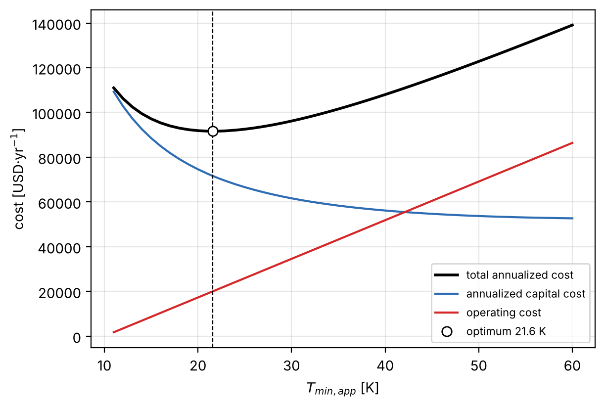
The sweep of the two-stream problem: the capital cost (blue) falls and the
operating cost (red) rises with T_min_app, and their sum (black) has
its minimum, 9.164e+04 USD/yr, at 21.59 K.#
The shells of this pair are large, so the capital cost falls smoothly. With
small streams it falls in steps: about one shell and tube each time the
shrinking area fills one fewer of 150 ft², or when the last one goes and
double pipes take the area. The least TAC then often lies just past such a
step, at the first T_min_app evaluated beyond it, and says more about
biosteam’s 150 ft² than about a trade-off of energy and capital; the sweep’s
'N_area_shells' and 'shell_type' (sweep.to_frame()) show where the
steps are. A network has such steps too, but where its own exchangers cross
150 ft².
The network against its targets#
network_report() compares the network the facility
synthesized with the targets of its streams, on the same options.
report = network_report(HXN)
target = report['targets']      # targets.summary() with the same options
print('                        network     target')
print(f"utility cost [USD/hr]   {report['utility_cost']:<10.2f}  {target['utility_cost']:.2f}")
print(f"units                   {report['N_units']:<10d}  {target['N_units']}")
print(f"area [m2]               {report['area']:<10.0f}  {target['area']:.0f}")
print(f"area, biosteam [m2]     {report['area_biosteam']:.0f}")
print(f"installed cost [USD]    {report['installed_cost']:<10.4g}  {target['installed_cost']:.4g}")
print(f"TAC [USD/yr]            {report['TAC']:<10.0f}  {target['TAC']:.0f}")
print('exchanger    area   biosteam [m2]')
for ID, (area, area_biosteam) in report['exchanger_areas'].items():
    print(f'{ID:<11}  {area:<5.0f}  {area_biosteam:.0f}')
                        network     target
utility cost [USD/hr]   1839.61     1839.61
units                   7           6
area [m2]               7462        5946
area, biosteam [m2]     5536
installed cost [USD]    2.184e+06   2.282e+06
TAC [USD/yr]            15072295    15088200
exchanger    area   biosteam [m2]
HX_1_2_hs    466    495
HX_0_2_hs    3097   3101
HX_1_4_hs    1      1
HX_1_3_hs    460    459
Util_2_cs    101    103
Util_0_hs    356    177
Util_1_hs    2983   1200
The network reaches the utility cost target, 1839.61 USD/hr: it is at MER, with the steam and chilled water that the targets allocate. That is not a rule: the utility cost target is the cost of biosteam’s agents placed on the grand composite curve, not a minimum, and a network at MER, which serves each stream with one agent at its outlet, can cost more (a costlier agent over a whole stream) or less (natural gas, which with biosteam’s default prices costs less per kJ than steam, heating a whole stream that ends above the hottest steam) than the target. The comparison of everything else needs care too, because a target is an estimate of an ideal network:
Area. The report’s
'area', 7462 m², re-sizes every exchanger of the network like the target sizes it: the same film coefficients, a correction factor of 1 and the integrated temperature difference along the streams’ profiles as the targets’ curves model them. On that basis the network needs more area than the 5946 m² target, as it should with equal film coefficients and the same utilities. biosteam’s own sizing, 5536 m² ('area_biosteam'), is lower still, mostly because it takes an overall coefficient of 1.0 kW/m²/K for condensing steam against a boiling stream (the steam heatersUtil_0_hsandUtil_1_hs: 177 and 1200 m² instead of 356 and 2983 m²), and because its terminal log-mean temperature difference overstates the mean driving force of a glide; it also applies a correction factor for its shells and sizes utility exchangers on the utility side duty. Because biosteam sizes on the terminal temperature differences only, an exchanger whose profiles cross inside it keeps a finite'area_biosteam', while its'area', and so the network’s, is infinite, with aRuntimeWarningnaming it. This happens when biosteam heats cooling water to its limit, 324.82 K, against a stream that condenses a little below that, as in a vacuum condenser: the utility’s line crosses the condensing stretch (see the Notes ofnetwork_report()).Units. The network has 7 exchangers against an estimate of 6 because it has a loop. Above the pinch, the bottoms cooler
D1_H1heats both the reboiler (HX_0_2_hs) and the flash’s feed heater (HX_1_2_hs), and each of these also has its own steam heater (Util_0_hsandUtil_1_hs), so the four exchangers close a loop: reboiler,D1_H1, feed heater, steam and back to the reboiler. Euler’s S - 1 counts the steam as one stream however many streams it heats, and assumes the matches of a region form no loop. The estimate can be wrong both ways: a balanced subset of streams needs fewer units, and each loop needs one more, whether a repeated match between two streams (two branches of a split stream meeting the same stream make one too) or, as here, two streams linked both through process matches and through a shared utility.Cost. The installed cost and the TAC of the network (2.184e+06 USD and 15072295 USD/yr) are biosteam’s, on biosteam’s areas, and here they are below the targets’ (2.282e+06 USD and 15088200 USD/yr), which divide a larger area into equal shells. Neither is a bound on the other.
The report’s 'targets' is summary() with the
same options, and the network and its targets are priced over the same
operating hours (the system’s, if it has them, else 8000 h/yr);
exchanger_areas gives both areas of each exchanger, which is
where a gap between the network and its target can be traced. The
synthesis itself does not optimize area, capital or total cost: it reaches
MER first and then keeps the number of exchangers low. Supertargeting is how
to choose the T_min_app it synthesizes at.
Where to next#
Key Concepts – the multiple-utility rule, the area, units and cost targets, the sweep, and the limits of each.
Targeting and supertargeting (hensmith.targeting) – every function, class and option of
hensmith.targeting.